Biometrical Genetics Workflow (bioflow)

The OneCGIAR biometrical genetics workflow or pipeline has been built to access methods for understanding or using evolutionary forces (mutation, gene flow, migration and selection) such as automatic state-of-the-art genetic evaluation (selection force) in decision-making. Designed to be database agnostic, it can retrieve data from the available phenotypic-pedigree databases (EBS, BMS, BreedBase), genotypic databases (GIGWA), and environmental databases (NASAPOWER), and carry the analytical procedures.

Version Control Technology

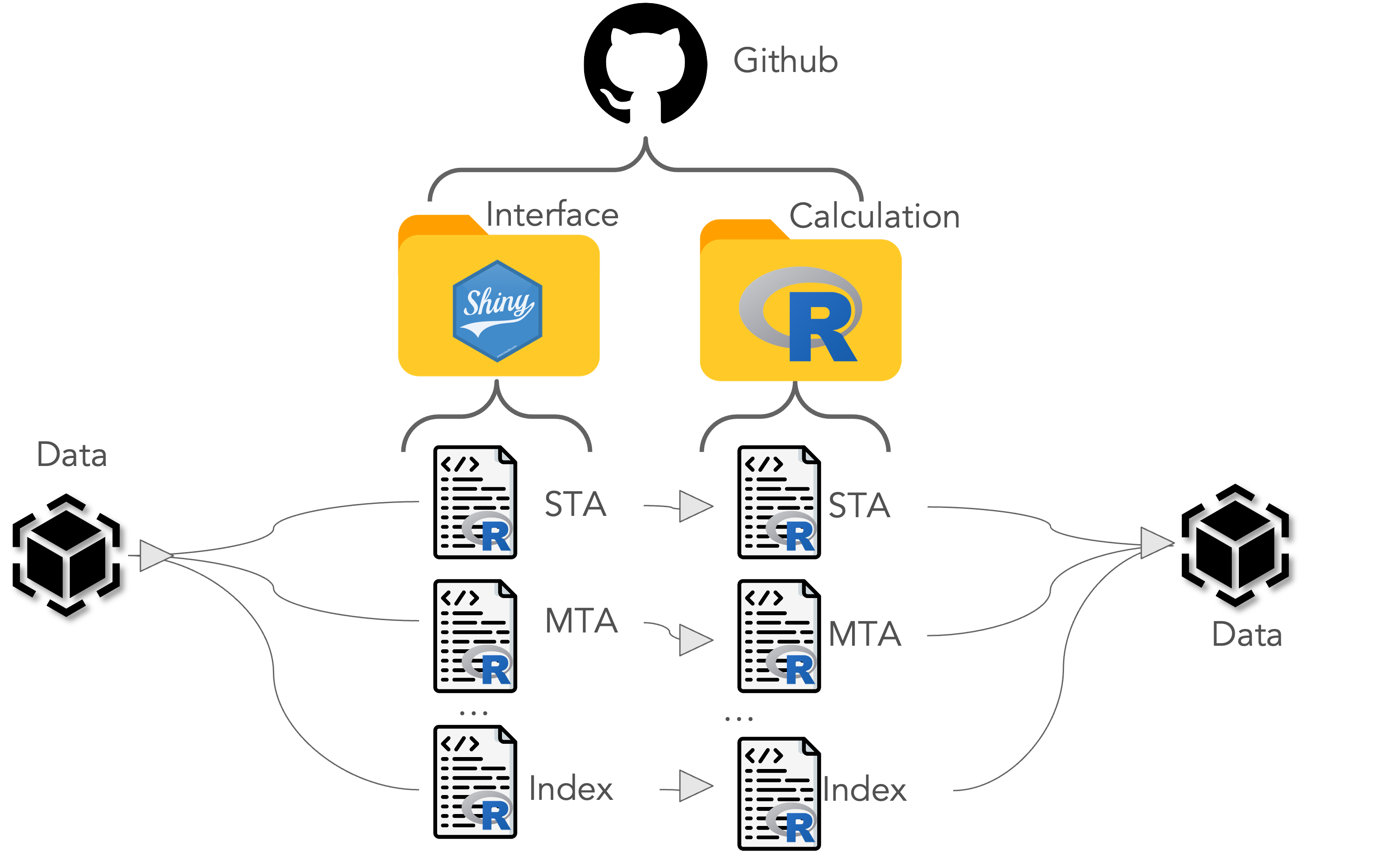
Our front and back end code is stored in Github to ensure team collaboration and quick fixes and improvement.

Developing Environment (IDE)

Our team uses R studio to develop packages, functions and pipelines for easy testing. In addition, the interface is developed using the shiny technology under the golem framework.

Data Storage Technology

The data extracted and produced is stored using an AWS-S3 container for flexibility and interoperability with other systems.

Deployment Technology

We use the docker technology to ensure the stability of our software and ensure the version control of our analytical pipeline.

Contributors of Analytical Modules

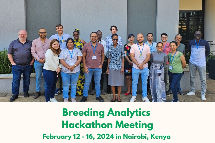
All CGIAR centers with Biometrics capacity have contributed to the design of the breeding analytics platform and currently work in developing analytical modules. Want to contribute? Contact us.

Team Activities

Team Members across Centers

ABI: Christian Werner (C.WERNER@cgiar.org), Dorcus Gemenet (d.gemenet@cgiar.org)

AfricaRice: Aubin Amagnide (A.Amagnide@cgiar.org)

CIAT: Sergio Cruz (S.Cruz@cgiar.org), Christian Cadena (C.C.Cadena@cgiar.org)

CIMMYT: Keith Gardner (K.GARDNER@cgiar.org), Angela Pacheco (r.a.pacheco@cgiar.org), Juan Burgueno (j.burgueno@cgiar.org), Abishek Rathore (ABHISHEK.RATHORE@cgiar.org), Roma Das (r.das@cgiar.org)

CIP: Bert de Boeck (B.DeBoeck@cgiar.org), Raul Eizaguirre (r.eyzaguirre@cgiar.org)

ICARDA: Khaled Al-Shamaa (K.EL-SHAMAA@cgiar.org)

ICRISAT: Anitha Raman (Anitha.raman@icrisat.org)

IITA: Ibnou Dieng (i.dieng@cgiar.org)

IRRI: Alaine Guilles (a.gulles@irri.org), Justine Bonifacio (j.bonifacio@irri.org), Daniel Pisano(d.pisano@irri.org), Leilani Nora (l.nora@irri.org)

Other Giovanny Covarrubias-Pazaran (covaruberpaz@gmail.com)

Contact us

Please use the following link (BIOFLOW Github Support Desk) to reach our Help Desk and send us your question or request.

Local installation

If you wish to install bioflow locally in your computer you have two options; 1) install it as an R library, or 2) download the bioflow portable for Windows systems.

The option 1) to install it as an R library requires to run the following three lines in your R or R studio console:

remotes::install_github('Breeding-Analytics/bioflow')

library(bioflow)

bioflow::run_app()

The first line will install bioflow as an r package in your computer. The second line will call the library/application to the environment. And the third line will start the application.

The option 2) to have a portable version of bioflow in an USB or computer is only functional for Windows and requires to just download it from Github

https://github.com/Breeding-Analytics/bioflowPortable

Additional instructions are available in the website above.

How to contribute to bioflow?

We do generate and maintain our code in Github. If you want to contribute you can clone the repository and use the sample data object to generate 2 files; 1) an R script with a function that uses as input the data object, performs your desired calculations, and returns the same data object. This R function file should be pushed to the cgiarPipeline package, 2) an R script for the shiny interface that uses behind the scenes the R function. This file should be pushed to the bioflow package. If you are only comfortable developing the R pipeline function and need support wit the interface contact us to support you.

Frequently asked questions

Why breeding analytics is important for my breeding program?

There are three main areas where breeding analytics is relevant for your organization (among others):

Parental selection: The selection for complex traits managed by hundreds or thousands of genes requires more than a trained eye. Biometrical genetics models allow to dissect the genetic signal from the environmental effects to allow the select parents with high breeding value. Together with selection indices and optimal contribution, breeding analytics guarantee greater genetic gains for complex traits compared to mass selection (visual selection).

Product development: Complex target population of environments require the proper understanding of genotype by environment interactions, and stability and sensitivity of materials to the different environmental conditions to be faced by the farmers. Biometrical genetics models can derive the sensititvity and stability of materials in few paramters and visualizations that guarantee the advacement of better and more stable products compared to classical approaches.

Trait discovery and introgression: Biometrical genetics offer a variety of linear and non-linear models to idenify genes behind traits of human interest. In addition, biometrical procedures make more efficient the introgression of beneficial alleles in terms of resources like time and cost.

What is different between bioflow and other platforms?

The strength of bioflow compared to other platforms is our flexible data structure that allows the transfer of data among different applications/modules. This way we can decouple or make the modules independent, so different biometricians can work in different modules without dependency on another. Certain modules depend on the results of another module (e.g., two stage analysis) but still certain level of independence exist.

Download Glossary

Data Retrieval and Saving

The first step in a pipeline consists in being able to retrieve phenotypic, genotypic, environmental information to be cleaned and analyzed with the different modules available. This section also allows to save the retrieved and analyzed data as an .RData object that can be later uploaded.

References:

Becker, R. A., Chambers, J. M. and Wilks, A. R. (1988) The New S Language. Wadsworth & Brooks/Cole.

Object Source*:

Browse...

Tutorial

Phenotype metadata

Storing place*:

Tutorial

Name assigned to the analysis object

Save object

What do we mean by quality assurance?

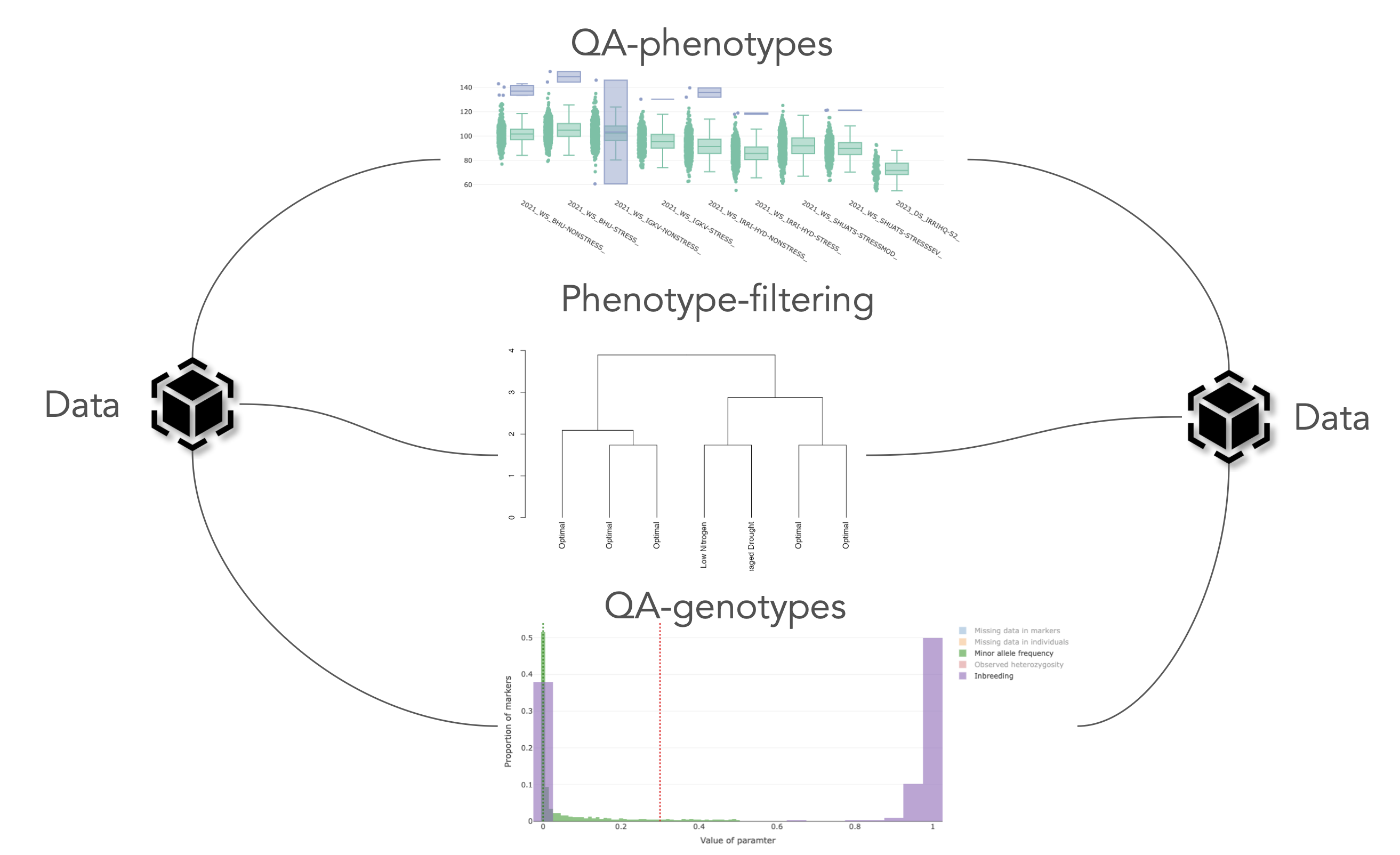
The analytical modules available expect good quality data to draw meaningful conclusions. Quality controls for phenotypes and genotypes are provided to filter and tag records that can lead to difficult interpretations.

The 'QA for phenotypes' modules allow the identification of outliers and filtering records based on indication columns.

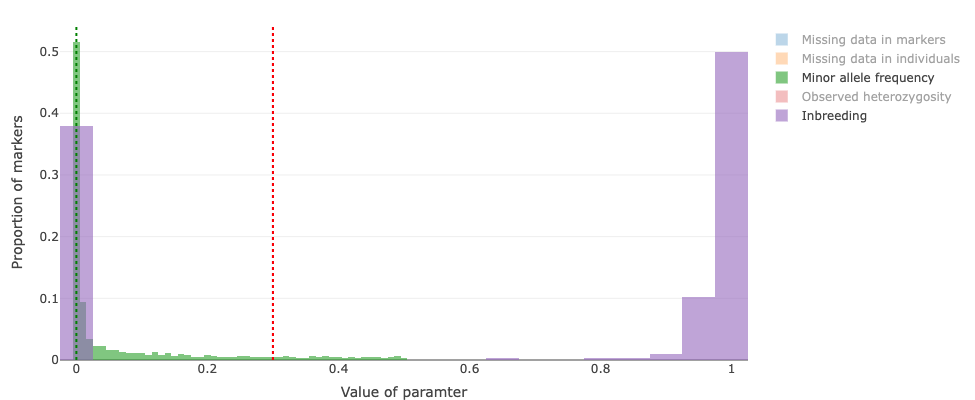
The 'QA for markers' module allows the identification of markers and individuals with high levels of missing data, minor allele frequency, heterozigosity and inbreeding.

Raw Phenotype Outlier Detection Module

Data Status (wait to be displayed):

Load example dataset

Details

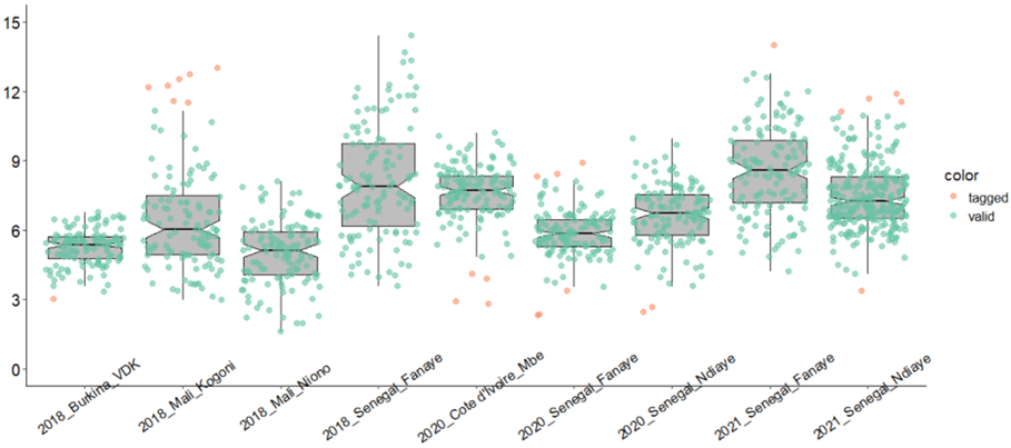
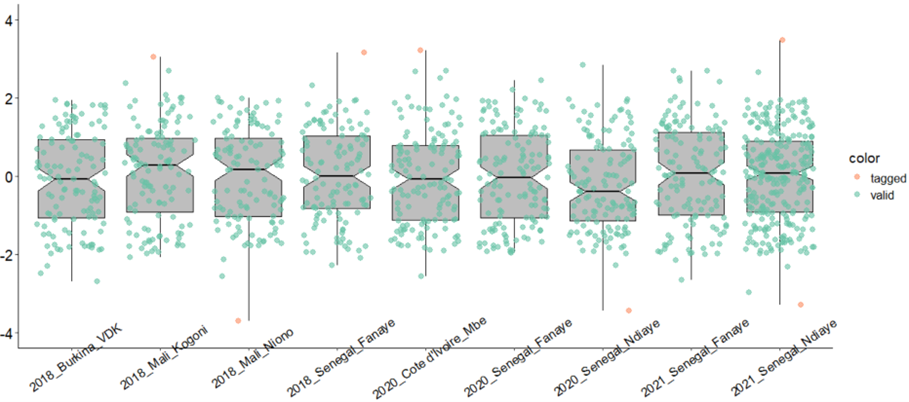
The first step in genetic evaluation is to ensure that input phenotypic records are of good quality. This option aims to allow users to select outliers based on plot whiskers and absolute values. The way arguments are used is the following:

Trait(s) to QA.- Trait(s) to apply jointly the parameter values in the grey box.

Outlier coefficient.- this determines how far the plot whiskers extend out from the box. If coef is positive, the whiskers extend to the most extreme data point which is no more than coef times the length of the box away from the box. A value of zero causes the whiskers to extend to the data extremes (and no outliers be returned).

References

Tukey, J. W. (1977). Exploratory Data Analysis. Section 2C.

McGill, R., Tukey, J. W. and Larsen, W. A. (1978). Variations of box plots. The American Statistician, 32, 12–16. doi:10.2307/2683468.

Velleman, P. F. and Hoaglin, D. C. (1981). Applications, Basics and Computing of Exploratory Data Analysis. Duxbury Press.

Set trait(s) & threshold
Run analysis

Trait(s) to QA

IQR coefficient

Visual aid (click on the '+' symbol on the right to open)

The visualizations of the input-data located below will not affect your analysis but may help you pick the right input-parameters to be specified in the grey boxes above.

Trait to visualize

Plot transparency

x-axis font size

Include x-axis labels

Analysis Name (optional)

Dashboard

Download dashboard

Genetic Markers Curation Module

Data Status (wait to be displayed):

Load example dataset

Details

When genetic evaluation is carried using genomic data, we need to ensure the quality of genetic markers. This option aims to allow users to identify bad markers or individuals given certain QA parameters. The way arguments are used is the following:

Threshold for missing data in markers.- this sets a threshold for how much missing data in a marker is allowed. Any marker with more than this value will be marked as a column to be removed in posterior analyses. Value between 0 and 1.

Threshold for missing data in individuals.- this sets a threshold for how much missing data in an individual is allowed. Any individual with more than this value it will be marked as a row to be removed in posterior analyses. Value between 0 and 1.

Minor allele frequency.- this sets a lower threshold for what is the minimum allele frequency allowed in the dataset. If lower than this value it will be marked as a column to be removed in posterior analyses. Value between 0 and 1.

Threshold for heterozygosity in markers.- this sets an upper threshold for what is the maximum level of heterozygosity allowed in the markers. If greater than this value it will be marked as a column to be removed in posterior analyses. Value between 0 and 1. For example, a line dataset should not have markers with high heterozigosity.

Threshold for inbreeding in markers.- this sets an upper threshold for what is the maximum level of inbreeding allowed in the markers. If lower than this value it will be marked as a column to be removed in posterior analyses. Value between 0 and 1.

Additional settings:

Imputation method.- method to impute missing cells. Median is the only method currently available.

Ploidy.- number of chromosome copies. This value is important to compute some of the paramters. Default is 2 or diploid.

References

Tukey, J. W. (1977). Exploratory Data Analysis. Section 2C.

Velleman, P. F. and Hoaglin, D. C. (1981). Applications, Basics and Computing of Exploratory Data Analysis. Duxbury Press.

Set thresholds
Run analysis

Upper threshold for missing data in markers (> will be removed)

Upper threshold for missing data in individuals(> will be removed)

Upper threshold for minor allele frequency (< will be removed)

Upper threshold for heterozygosity in markers (> will be removed)

Upper threshold for inbreeding in markers (> will be removed)

Visual aid (click on the '+' symbol on the right to open)

The visualizations of the input-data located below will not affect your analysis but may help you pick the right input-parameter values to be specified in the grey boxes above.

Analysis Name (optional)

Additional run settings (optional)...

Imputation method

Ploidy

Dashboard

Download dashboard

Trait transformations

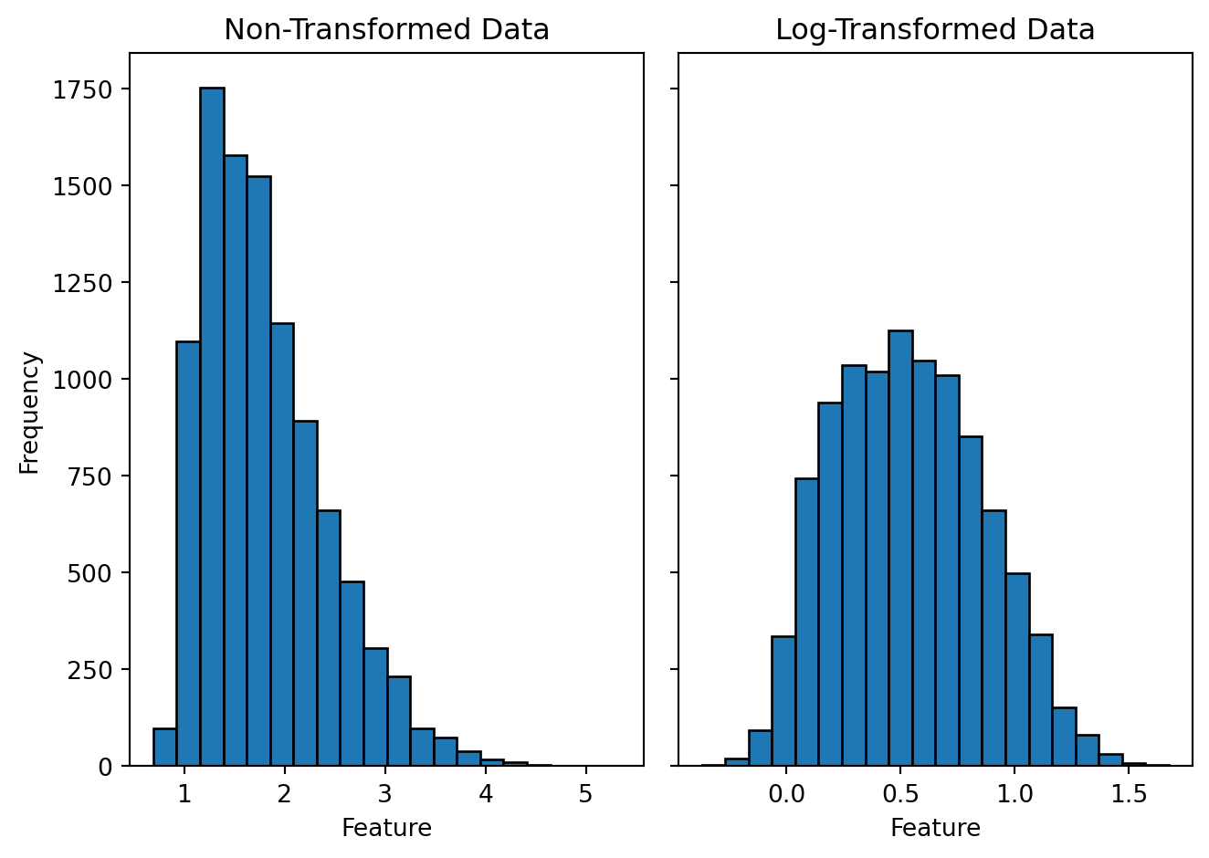
Traits of interest for biologist present a variety of scales and more important, different distributions. Although bioflow allows flexibility to fit models on traits that present different distributions other than normal, having the ability to transform certain traits present another opportunity to simplify the models. In adiition, sometimes scientist just need to create a new trait that is a linear transformation of others.

Bioflow currently offers few transformations such as log, square root, identity, among others.

References:

Becker, R. A., Chambers, J. M. and Wilks, A. R. (1988) The New S Language. Wadsworth & Brooks/Cole. (for log, log10 and exp.)

Image taken from https://dataalltheway.com/posts/001-data-transformation/index.html

Trait Transformation Module

Data Status (wait to be displayed):

Details

Some trait transformations are required when data starts to grow or presents modeling challenges. The current implementations include:

Conversion- The trait is transformed by a function such as cubic root, square root, log., etc..

Equalizing- a set of traits with different name are considered to be the same trait and the user needs to equalize them .

Balancing- a trait with numerical values in different units depending on the environment needs to be converted to same units across environments .

References

Software used

R Core Team (2021). R: A language and environment for statistical computing. R Foundation for Statistical Computing, Vienna, Austria. URL https://www.R-project.org/.

Input
Output

Input
Output

Trait(s) to equalize

Name for the new trait

Input
Output

Traits available

Name for the new trait

Formula to compute

Single Cross Marker Matrix Building Module

Data Status (wait to be displayed):

Load example dataset

Details

Hybrid breeding based on single-cross of lines allows the genotyping of only the parental lines and the consequent formation of single-cross marker matrices. The idea is that the user provides the marker information from the parental lines and has uploaded a pedigree of the phenotypic dataset. The marker profiles of the possible cross combinations will be computed based on the availability of the marker information. Some of the parameters required are:

Batch size to compute- the number of hybrids to build in each batch. Building all hybrids at once can be computationally intensive and unnecesary. The default value is 1000 hybrids per batch.

Compute all possible hybrids?- an indication to know if only the marker-profiles for the hybrids present in the pedigree dataset should be computed or marker-profiles for all cross combinations should be created. This should be used carefully when the number of males and females in the pedigree file is big.

Example

References

Nishio M and Satoh M. 2014. Including Dominance Effects in the Genomic BLUP Method for Genomic Evaluation. Plos One 9(1), doi:10.1371/journal.pone.0085792

Su G, Christensen OF, Ostersen T, Henryon M, Lund MS. 2012. Estimating Additive and Non-Additive Genetic Variances and Predicting Genetic Merits Using Genome-Wide Dense Single Nucleotide Polymorphism Markers. PLoS ONE 7(9): e45293. doi:10.1371/journal.pone.0045293

Software used

R Core Team (2021). R: A language and environment for statistical computing. R Foundation for Statistical Computing, Vienna, Austria. URL https://www.R-project.org/.

Covarrubias-Pazaran G. 2016. Genome assisted prediction of quantitative traits using the R package sommer. PLoS ONE 11(6):1-15.

QA stamp to apply to markers

Visual aid (click on the '+' symbol on the right to open)

The visualizations of the input-data located below will not affect your analysis but may help you pick the right input-parameters to be specified in the grey boxes above.

Batch size to compute

Visual aid (click on the '+' symbol on the right to open)

The visualizations of the input-data located below will not affect your analysis but may help you pick the right input-parameters to be specified in the grey boxes above.

Compute all possible hybrids?

Visual aid (click on the '+' symbol on the right to open)

The visualizations of the input-data located below will not affect your analysis but may help you pick the right input-parameters to be specified in the grey boxes above.

Number of mothers

Number of fathers

Analysis Name (optional)

Data

Download Genotypic data

What do we mean by quality assurance?

The 'QA for phenotypes' modules allow the identification of outliers and filtering records based on indication columns.

The 'QA for markers' module allows the identification of markers and individuals with high levels of missing data, minor allele frequency, heterozigosity and inbreeding.

Environment-Pheno Filtering Module

Data Status (wait to be displayed):

Details

The first step in genetic evaluation is to ensure that input phenotypic records are of good quality. This option allows users to filter (more concretely tag records for exclusion) specific years, seasons, countries, locations, etc. from the posterior analyses. This is just an optional module that most users will not require. The way arguments are used is the following:

label.- the different columns to subset the phenotypic dataset to exclude certain years, seasons, countries, locations, trials, or environments for certain traits.

References

Tukey, J. W. (1977). Exploratory Data Analysis. Section 2C.

Velleman, P. F. and Hoaglin, D. C. (1981). Applications, Basics and Computing of Exploratory Data Analysis. Duxbury Press.

Trait to filter

Years to keep

Seasons to keep

Countries to keep

Locations to keep

Trials to keep

Environments to keep

Settings...

Maximum #of genotypes allowed (trials with more will be removed)

Visual aid (click on the '+' symbol on the right to open)

The visualizations of the input-data located below will not affect your analysis but may help you pick the right input-parameter values to be specified in the grey boxes above.

Apply same filter to other trait(s)?

Trait(s) to apply the same filters

Analysis Name (optional)

Dashboard

Download dashboard

Experimental Design Factor Filtering Module

Data Status (wait to be displayed):

Details

Sometimes is required to set to missing experimental design factors that we are aware that are not correctly saved in the databases. Although the tight solution would be to fix this information in the original database, a pragmatic approach is to set certain factors from an especific environment to missing so it is ignored in the model fitting or any other analytical module using this information.

Editing table- there is not much complexity of how to use this module. There is a table with a column for each experimental design factor and a row for each environment. By default this table is filled with the number of levels wherever this information is available. If the user wants to silence a particular factor it just needs to double click in the cell and set the value to zero.

Pick factor(s)
Run analysis

The experimental design factors (columns) present in a particular environment (rows) are displayed in the table below. Please double click in any cell (environment by factor combination) that you would like to silence by setting the value to zero. Then run the analysis to save those modifications for posterior analyses.

Visual aid (click on the '+' symbol on the right to open)

The visualizations of the input-data located below will not affect your analysis but may help you pick the right input-parameter values to be specified in the grey boxes above.

Heatmap to explore the spatial distribution of factors and traits. Row and column information need to be mapped for this visualization to properly display.

Environment to visualize

Color field by

Text cells by

Analysis Name (optional)

Dashboard

Download dashboard

Data Consistency QA Module

Data Status (wait to be displayed):

Load example dataset

Details

Some additional checks for data consistency are benefitial to ensure a high quality analysis. These can include:

Check names- The onthology for some crops is particularly important. This tab allows to check this to a reference onthology.

Check traits- Checking the relationships between traits is particularly useful to identify issues.

Tag inconsistencies- Once inconsistencies are identified, is important to tag them for posterior management in the analytical modules.

References

Software used

R Core Team (2021). R: A language and environment for statistical computing. R Foundation for Consisttistical Computing, Vienna, Austria. URL https://www.R-project.org/.

Select your crop filter:

IQR coefficient

Design for residuals calculation

Residual threshold

Visual aid (click on the '+' symbol on the right to open)

The visualizations of the input-data located below will not affect your analysis but may help you pick the right input-parameters to be specified in the grey boxes above.

Matrix of issues (transposed dataset).

Records

Columns/traits

Analysis Name (optional)

Dashboard

Download dashboard

What is genetic evaluation?

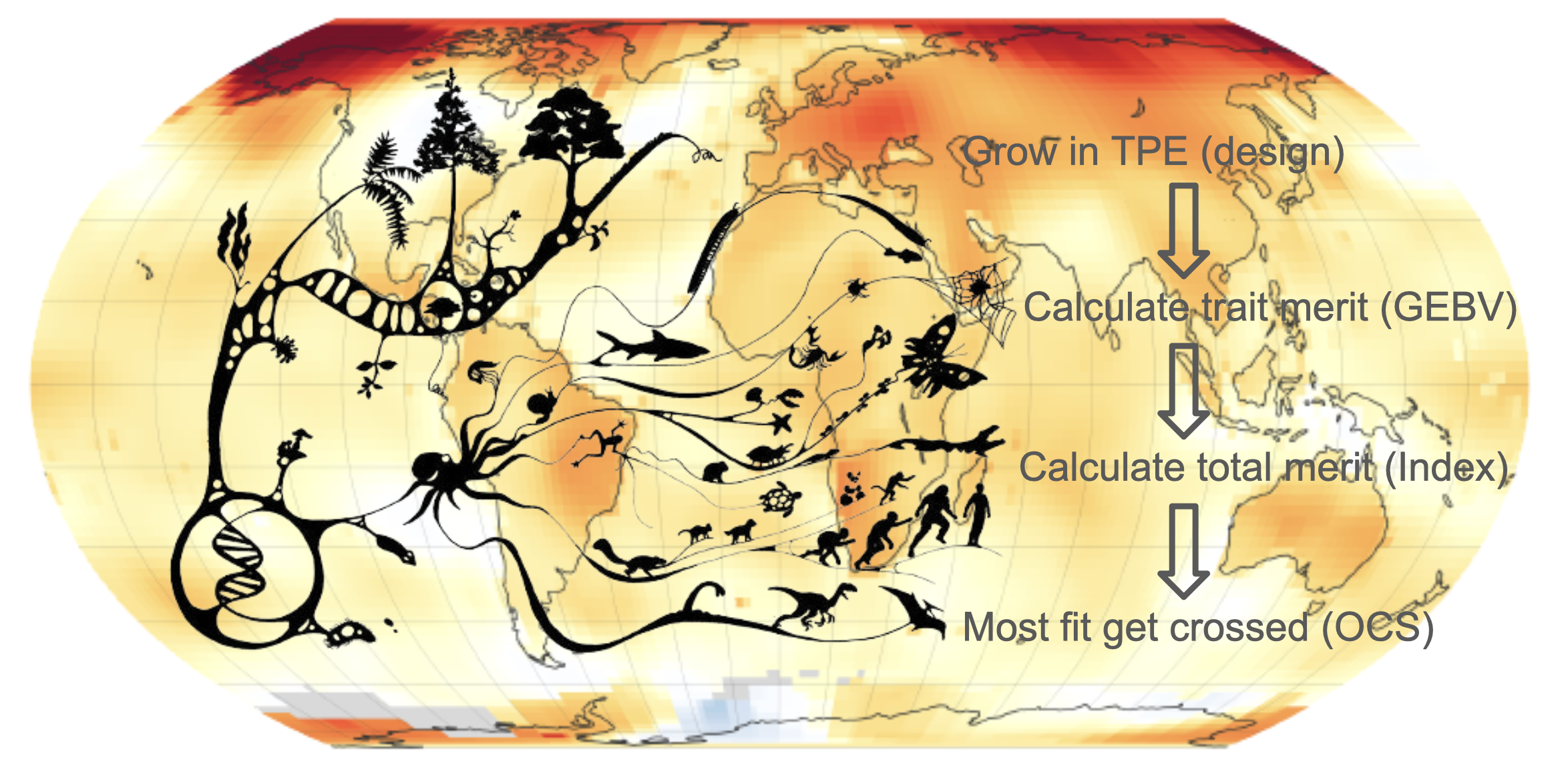
Genetic evaluation is the process to dissect the genetic signal from the phenotypic records to estimate surrogates of genetic value [i.e., breeding values (BV), general combining ability (GCA), total genetic value(GV)] in order to apply artificial selection using such estimates and increase the allele frequencies of genes affecting the expression of the traits of interest in a particular target population of environments (TPE).

The genetic evaluation approach used in bioflow is the so-called 'two-stage'. After cleaning the raw phenotypic records from outliers and typos the data is analysed environment by environment to remove the spatial noise and extract genotype BLUEs and standard errors (stage 1). This could be followed by an alternative QA step to identify outliers using standardized residuals. The genotype BLUEs from the first stage (and optionally genetic markers, pedigree information, and environmental data) are used to fit a multi-environment analysis to produce across-environment surrogates of genetic merit for each trait (e.g., BLUPs, GBLUP, etc.) and stability surrogates across environments.

It is recommended to use the trait-BVs to produce a selection index (net merit) that can be used in one of two alternatives; 1) select parents with high net merit for the next crossing block, or 2) simulate and select predicted crosses with the highest net merit using the optimal cross selection (OCS) procedure based on contribution theory.

Additional notes:

For a trait where you only have single replicate data (no replication within environment per genotype) and want to use pedigree or markers to separate the error from the genetic signal, you need to perform the single trial analysis first to move your single-replicate records per environment to the second stage where you can use your pedigree or marker information. Make sure you accept environments with H2=0 coming from the first stage since unreplicated environments or trial will be assumed to have H2=0.

Marker-Assisted Selection Module Using Selection Index Theory

Data Status (wait to be displayed):

Load example dataset

Details

The availability of genetic markers linked closely to QTLs allow to select directly for the fixation of the QTL without further phenotyping. When such markers exist you can use this module to select individuals that help to increase the frequency of the positive QTL-allele. Currently, the method consists in weighting each marker by 1-freq, where freq is the frequency of the positive QTL-allele. In addition, the user is allowed to multliply that first weight by a factor.The following parameters are enabled:

Markers to be used.- selection of genetic markers to be used for the verification process.

Desired dosages.- this is the way to set the direction on what allele should be selected (positive allele for the trait of interest). The allele shown in the slider is the reference allele picked in the transformation for the dosage matrix.

Relative weights for each marker.- relative values to apply to each marker denoting the multiplier applied to the 1-freq approach.

References

Liu, B. H. (2017). Statistical genomics: linkage, mapping, and QTL analysis. CRC press.

Velleman, P. F. and Hoaglin, D. C. (1981). Applications, Basics and Computing of Exploratory Data Analysis. Duxbury Press.

QA-geno stamp(s) to apply

Visual aid (click on the '+' symbol on the right to open)

The visualizations of the input-data located below will not affect your analysis but may help you pick the right input-parameters to be specified in the grey boxes above.

Marker(s) to use

Select all markers at once?

Visual aid (click on the '+' symbol on the right to open)

The visualizations of the input-data located below will not affect your analysis but may help you pick the right input-parameter values to be specified in the grey boxes above.

Markers to display

Ploidy of the organism

Visual aid (click on the '+' symbol on the right to open)

The visualizations of the input-data located below will not affect your analysis but may help you pick the right input-parameter values to be specified in the grey boxes above.

Analysis Name (optional)

Download dashboard

Single Trial Analysis Module

Data Status (wait to be displayed):

Load example dataset

Details

The genetic evaluation approach we use known as 'two-step' first analyze trait by trait and trial by trial to remove the spatial noise from experiments using experimental factors like blocking and spatial coordinates. Each trial is one level of the environment column (defined when the user matches the expected columns to columns present in the initial phenotypic input file). Genotype is fitted as both, fixed and random. The user defines which should be returned in the predictions table. By default genotype (designation column) predictions and their standard errors are returned. The way the options are used is the following:

Genetic evaluation unit.- One or more of the following; designation, mother, father to indicate which column(s) should be considered the unit of genetic evaluation to compute BLUEs or BLUPs in the single trial analysis step.

Traits to analyze.- Traits to be analyzed. If no design factors can be fitted simple means are taken.

Covariates.- Columns to be fitted as as additional fixed effect covariates in each trial.

Additional settings.-

Type of estimate.- Whether BLUEs or BLUPs should be stored for the second stage.

Number of iterations.- Maximum number of restricted maximum likelihood iterations to be run for each trial-trait combination.

Print logs.- Whether the logs of the run should be printed in the screen or not.

Note.- A design-agnostic spatial design is carried. That means, all the spatial-related factors will be fitted if pertinent. For example, if a trial has rowcoord information it will be fitted, if not it will be ignored. A two-dimensional spline kernel is only fitted when the trial size exceeds 5 rows and 5 columns. In addition the following rules are followed: 1) Rows or columns are fitted if you have equal or more than 3 levels, 2) Reps are fitted if you have equal or more than 2 levels, 3) Block (Sub-block) are fitted if you have equal or more than 4 levels.

References

Velazco, J. G., Rodriguez-Alvarez, M. X., Boer, M. P., Jordan, D. R., Eilers, P. H., Malosetti, M., & Van Eeuwijk, F. A. (2017). Modelling spatial trends in sorghum breeding field trials using a two-dimensional P-spline mixed model. Theoretical and Applied Genetics, 130, 1375-1392.

Rodriguez-Alvarez, M. X., Boer, M. P., van Eeuwijk, F. A., & Eilers, P. H. (2018). Correcting for spatial heterogeneity in plant breeding experiments with P-splines. Spatial Statistics, 23, 52-71.

Software used

R Core Team (2021). R: A language and environment for statistical computing. R Foundation for Statistical Computing, Vienna, Austria. URL https://www.R-project.org/.

Boer M, van Rossum B (2022). _LMMsolver: Linear Mixed Model Solver_. R package version 1.0.4.9000.

Pheno-modification stamp(s) to apply to the data

Visual aid (click on the '+' symbol on the right to open)

The visualizations of the input-data located below will not affect your analysis but may help you pick the right input-parameters to be specified in the grey boxes above.

Trait(s) to analyze

Covariable(s) (optional)

Alternative response distributions...

The Normal distribution is assumed as default for all traits. If you wish to specify a different trait distribution for a given trait double click in the cell corresponding for the trait by distribution combination and make it a '1'.

Visual aid (click on the '+' symbol on the right to open)

The visualizations of the input-data located below will not affect your analysis but may help you pick the right input-parameters to be specified in the grey boxes above.

Trait to visualize

Plot transparency

Genetic evaluation unit(s)

Additional run settings (optional)...

Estimate type

Number of iterations

Print log file?

Visual aid (click on the '+' symbol on the right to open)

The visualizations of the input-data located below will not affect your analysis but may help you pick the right input-parameters to be specified in the grey boxes above.

Summarize evaluation units by:

Analysis Name (optional)

Download dashboard

Model-Based Outlier Detection Module

Data Status (wait to be displayed):

Load example dataset

Details

The two-step approach of genetic evaluation allows to identify noisy records after the single trial analysis. This option aims to allow users to select model-based outliers based on plot whiskers and absolute values applied on conditional residuals. The way arguments are used is the following:

Trait(s) residuals to QA.- Trait(s) residuals to apply jointly the parameter values in the grey box.

References

Tukey, J. W. (1977). Exploratory Data Analysis. Section 2C.

McGill, R., Tukey, J. W. and Larsen, W. A. (1978). Variations of box plots. The American Statistician, 32, 12–16. doi:10.2307/2683468.

Velleman, P. F. and Hoaglin, D. C. (1981). Applications, Basics and Computing of Exploratory Data Analysis. Duxbury Press.

Set trait(s) & threshold
Run analysis

Trait(s) to QA

IQR coefficient

Visual aid (click on the '+' symbol on the right to open)

The visualizations of the input-data located below will not affect your analysis but may help you pick the right input-parameter values to be specified in the grey boxes above.

Preview of outliers that would be tagged using current input parameters above for trait selected.

Plot settings...

x-axis font size

Analysis Name (optional)

Dashboard

Download dashboard

Desire Selection Index Module

Data Status (wait to be displayed):

Load example dataset

Details

Genetic evaluation has as final purpose to select the individuals with highest genetic merit across all traits of interest. In order to select for multiple traits at the same time a selection index is preferred. This option aims to calculate a selection index using across-environment predictions from multiple traits based on user's desired change (used to calculate weights) and return a table of predictions with the index and the traits used for selection. The way the options are used is the following:

Traits to include in the index- Traits to be considered in the index.

Desire or base values.- Vector of values indicating the desired change in traits.

Scale traits.- A TRUE or FALSE value indicating if the table of traits should be scaled or not. If TRUE is selected, the values of the desire vector are expected to be expressed in standard deviations. If FALSE, the values of the desire vector are expected to be expressed in original-scale units.

References

Pesek, J., & Baker, R. J. (1969). Desired improvement in relation to selection indices. Canadian journal of plant science, 49(6), 803-804.

Ceron-Rojas, J. J., & Crossa, J. (2018). Linear selection indices in modern plant breeding (p. 256). Springer Nature.

Software used

R Core Team (2021). R: A language and environment for statistical computing. R Foundation for Statistical Computing, Vienna, Austria. URL https://www.R-project.org/.

MTA or MAS version(s) to find traits

Visual aid (click on the '+' symbol on the right to open)

The visualizations of the input-data located below will not affect your analysis but may help you pick the right input-parameters to be specified in the grey boxes above.

Trait(s) to analyze

Environment to use

Effect type to use

Entry type(s) to use

Scale traits for index?

Visual aid (click on the '+' symbol on the right to open)

The visualizations of the input-data located below will not affect your analysis but may help you pick the right input-parameters to be specified in the grey box in the left

Font size

Selected proportion for graphs

Metrics associated to the MTA stamp selected.

Parameter to visualize

Analysis Name (optional)

Additional run settings (optional)...

Print logs?

Download dashboard

Base Selection Index Module

Data Status (wait to be displayed):

Load example dataset

Details

This option (base index) aims to calculate a selection index using user's predefined weights and return a table of predictions with the index and the traits used for selection.

If relative economic values of each trait are available and acceptable, a base index can be used to improve multiple traits simultaneously. In this scenario, an index is calculated for each individual by using the phenotypic values (BLUPs) observed for each trait and assigning the economic values associated with each trait as the index coefficients. Assigning economic weights to traits is however a complex task, as it requires knowledge of various market variables such as prices and profit objectives.

If there are uncertainty on how to determine the economic weights, then an index based on the desired genetic gains for each trait is recommended

The way the options are used is the following:

Traits to include in the index- Traits to be considered in the index.

Base values.- Vector of values indicating the desired change in traits.

References

Brim, C. A., Johnson, H. W., & Cockerham, C. C. (1959). Multiple selection criteria in soybeans 1. Agronomy Journal, 51(1), 42-46.

Ceron-Rojas, J. J., & Crossa, J. (2018). Linear selection indices in modern plant breeding (p. 256). Springer Nature.

Software used

R Core Team (2021). R: A language and environment for statistical computing. R Foundation for Statistical Computing, Vienna, Austria. URL https://www.R-project.org/.

MTA version(s) to analyze

Visual aid (click on the '+' symbol on the right to open)

The visualizations of the input-data located below will not affect your analysis but may help you pick the right input-parameter values to be specified in the grey boxes above.

Trait(s) to analyze

Analysis Name (optional)

Additional run settings (optional)...

Print logs?

Download dashboard

Options:
OCS
GPCP

Optimal Cross Selection Module

Data Status (wait to be displayed):

Load example dataset

Details

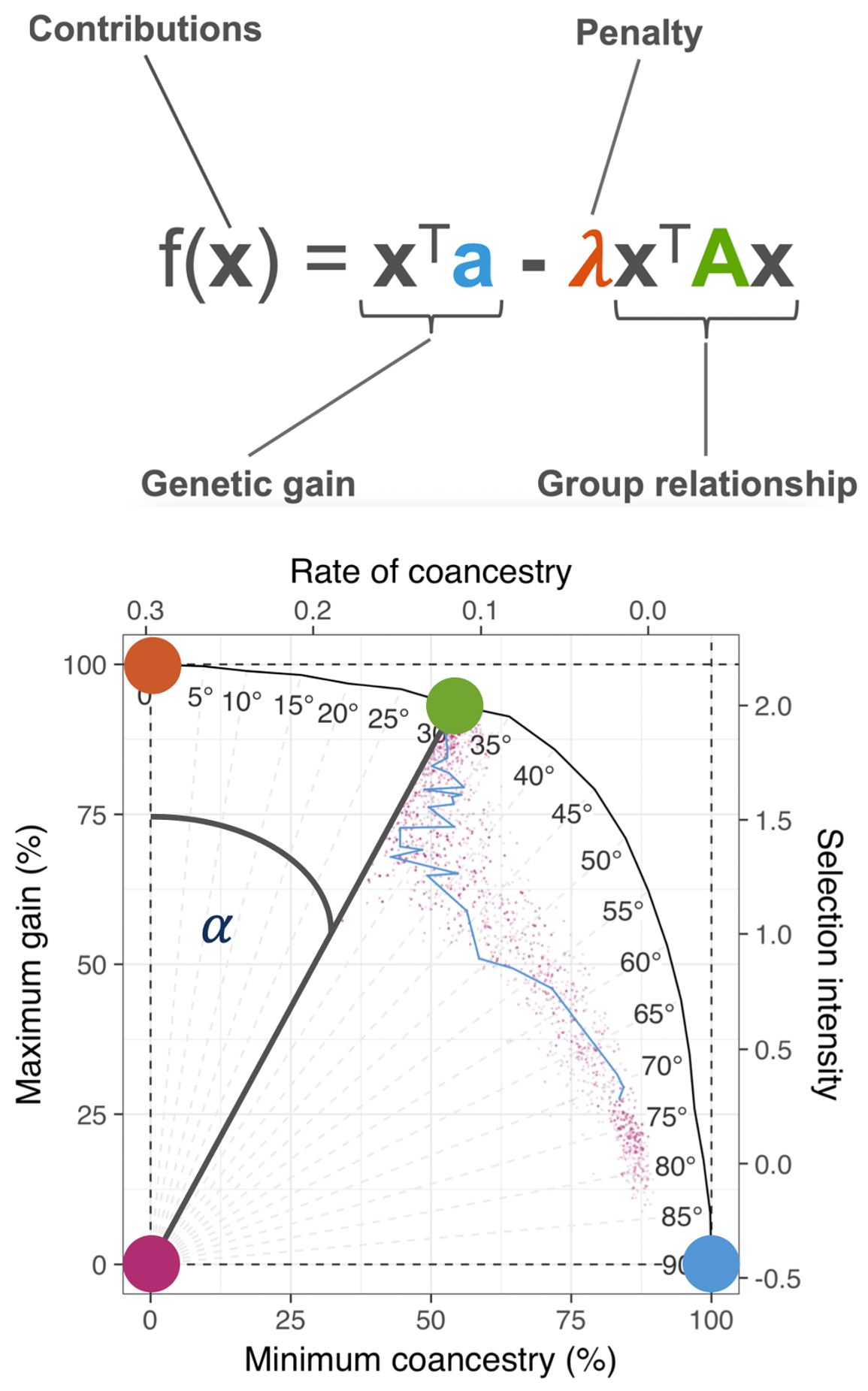
A new generation of individuals with higher genetic merit can be produced selecting the top individuals or selecting directly the best crosses. This option aims to optimize the new crosses given a desired trade-off between short-term gain(performance) and long-term gain (genetic variance). The way the options are used is the following:

Trait for cross prediction.- Trait to be be used for predicting all possible crosses (an index is suggested).

Entry types to use.- Which entry types should be used in the algorithm.

Number of crosses.- Number of top crosses to be selected.

Target angle.- Target angle defining the trade-off between performance and diversity. Zero degrees is weighting strongly towards performance. Ninety degrees is weighting strongly towards diversity.

Additional settings.-

Maximum number of top individuals to use.- The complexity and computation time of the algorithm scales up with greater number of individuals used for predicted crosses. This arguments applies a filter to only use the top N individuals for the trait of interest.

Stopping criteria.- Maximum number of runs (iterations) without change in the genetic algorithm.

Relationship to use.- One of the following; GRM, NRM single-step relationship matrix.

Environment to use.- If the user wants to use predictions from an specific environment. In NULL all are used.

Notes.- Consider that the predictions table in this particular case is different. In this case, the 'predictedValue' column refers to the expected value of the cross, 'stdError' is the average inbreeding of the cross, and 'rel' has the genetic algorithm value (lower the better).

References

Kinghorn, B. (1999). 19. Mate Selection for the tactical implementation of breeding programs. Proceedings of the Advancement of Animal Breeding and Genetics, 13, 130-133.

https://alphagenes.roslin.ed.ac.uk/wp/wp-content/uploads/2019/05/01_OptimalContributionSelection.pdf?x44213

Woolliams, J. A., Berg, P., Dagnachew, B. S., & Meuwissen, T. H. E. (2015). Genetic contributions and their optimization. Journal of Animal Breeding and Genetics, 132(2), 89-99.

Software used

R Core Team (2021). R: A language and environment for statistical computing. R Foundation for Statistical Computing, Vienna, Austria. URL https://www.R-project.org/.

https://github.com/gaynorr/QuantGenResources

Index version to analyze

Visual aid (click on the '+' symbol on the right to open)

The visualizations of the input-data located below will not affect your analysis but may help you pick the right input-parameters to be specified in the grey boxes above.

Trait(s) to optimize

Effect type to use

Entry type to use in optimization

Visual aid (click on the '+' symbol on the right to open)

The visualizations of the input-data located below will not affect your analysis but may help you pick the right input-parameters to be specified in the grey boxes above.

Trait to visualize

Group by

Include x-axis labels

x-axis font size

Number of crosses

Target angle

Relationship to use

Visual aid (click on the '+' symbol on the right to open)

The visualizations of the input-data located below will not affect your analysis but may help you pick the right input-parameters to be specified in the grey boxes above.

Analysis Name (optional)

Additional run settings (optional)...

Maximum number of top individuals to use

Stopping criteria (#of iterations without change)

Environment to use

Print logs?

Download dashboard

What do we mean by selection history?

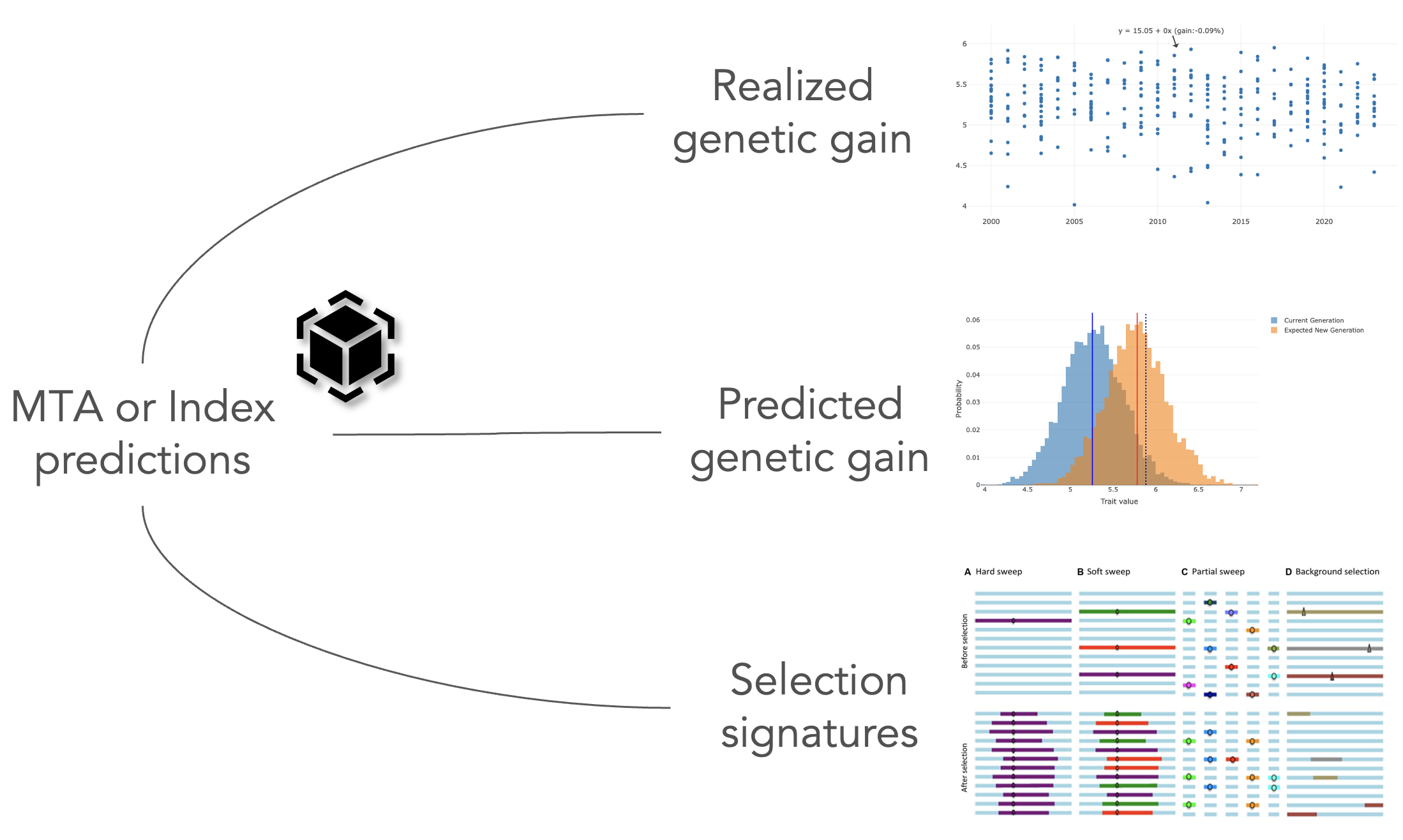
The selection history modules allow the user to calculate genetic gain or population mean and variance changes across generations for traits of interest. In addition, it also allows to calculate the so called 'predicted' genetic gain which are parameters such as selection intensity, accuracy, genetic variance and cycle time in order to monitor the practices and operations of the breeding program along with the management of the genetic variability.

The approach used in bioflow consist in using estimates of genetic value from the multi-trait analysis for a particular trait or a selection index of traits.

The 'selection signatures' module allow to identify regions of the genome that have experienced artificial or natural selection.

Realized Genetic Gain Module

Data Status (wait to be displayed):

Load example dataset

Details

In order to monitor the efficacy of genetic evaluation across cycles of selection, the realized genetic gain is the preferred process. This option aims to calculate the realized genetic gain using the methods from Mackay et al. (2011). The method uses across-environment means from multiple years of data that have been adjusted based on a good connectivity to then fit a regression of the form means~year.of.origin. In case the means used are BLUPs these can be deregressed. The way the options are used is the following:

Method.- One of the following; Mackay et al. (2011) or Laidig et al. (2014).

Trait(s) to use.- Trait to be be used for realized genetic gain estimation (an index is suggested).

Years of origin to use.- Selection of the years of origin associated to the tested material to use in the calculation.

Entry types to use.- A selection of entry types to use for the realized genetic gain calculation.

Deregress weight.- Should any weight be applied to the deregressed value (not recommended but available).

Partition the data?.- When very few years of data are present this option will allow the user to calculate the gain for all 2-year combinations and then average these rates.

Deregress estimates- Should we deregress the estimates by dividing over the reliability before performing the realized genetic gain calculation.

References

Mackay, I., Horwell, A., Garner, J., White, J., McKee, J., & Philpott, H. (2011). Reanalyses of the historical series of UK variety trials to quantify the contributions of genetic and environmental factors to trends and variability in yield over time. Theoretical and Applied Genetics, 122, 225-238.

Laidig, F., Piepho, H. P., Drobek, T., Meyer, U. (2014). Genetic and non-genetic long-term trends of 12 different crops in German official variety performance trials and on-farm yield trends. Theoretical and Applied Genetics, 127, 2599-2617.

Rutkoski, J. E. (2019). A practical guide to genetic gain. Advances in agronomy, 157, 217-249.

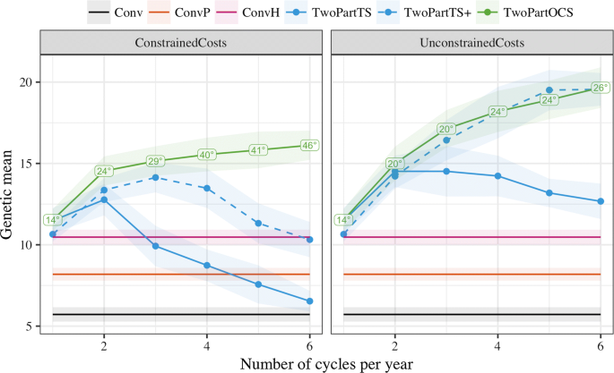
Gorjanc, G., Gaynor, R. C., Hickey, J. M. (2018). Optimal cross selection for long-term genetic gain in two-part programs with rapid recurrent genomic selection. Theoretical and applied genetics, 131, 1953-1966.

Software used

R Core Team (2021). R: A language and environment for statistical computing. R Foundation for Statistical Computing, Vienna, Austria. URL https://www.R-project.org/.

Data version to analyze

Method

Mackay

Piepho

Visual aid (click on the '+' symbol on the right to open)

The visualizations of the input-data located below will not affect your analysis but may help you pick the right input-parameter values to be specified in the grey boxes above.

Trait(s) to use

Visual aid (click on the '+' symbol on the right to open)

The visualizations of the input-data located below will not affect your analysis but may help you pick the right input-parameter values to be specified in the grey boxes above.

Trait to visualize regression over years.

Year(s) of origin to use

Environment to use

Effect type(s) to use

Entry type(s) to use

Visual aid (click on the '+' symbol on the right to open)

The visualizations of the input-data located below will not affect your analysis but may help you pick the right input-parameter values to be specified in the grey boxes above.

Trait to visualize regression over years.

Analysis Name (optional)

Additional run settings (optional)...

Deregression weight

Top proportion individuals to keep per year of origin

Partitioned regression

Number of entries per environment to sample

Number of bootstrapping per samples

Print logs?

#Years rule applied?

Download dashboard

Predicted Genetic Gain Module

Data Status (wait to be displayed):

Load example dataset

Details

In order to monitor the efficacy of genetic evaluation in the current cycle of selection the predicted genetic gain formula is used. This option aims to calculate the predicted genetic gain from the classical breeders' equation R = i*r*s being R the response to selection, i the selection intensity, r the selection accuracy, s the genetic standard deviation. The way the options are used is the following:

Trait(s) to use.- Trait to be be used for calculating the predicted genetic gain parameters.

Environment(s) to use.- Environments-data to be used from the input file.

Proportion selected.- Proportion of parents to be selected in order to calculate the selection intensity.

References

Lush, J. L. (2013). Animal breeding plans. Read Books Ltd.

Mrode, R. A. (2014). Linear models for the prediction of animal breeding values. Cabi.

Software used

R Core Team (2021). R: A language and environment for statistical computing. R Foundation for Statistical Computing, Vienna, Austria. URL https://www.R-project.org/.

STA version to analyze

Visual aid (click on the '+' symbol on the right to open)

The visualizations of the input-data located below will not affect your analysis but may help you pick the right input-parameter values to be specified in the grey boxes above.

Trait(s) to use

Do analysis by:

Assumed percentage selected (%)

Visual aid (click on the '+' symbol on the right to open)

The visualizations of the input-data located below will not affect your analysis but may help you pick the right input-parameter values to be specified in the grey boxes above.

Trait to visualize

Parameter to visualize

Analysis Name (optional)

Download dashboard

Module under construction.

What is gene discovery?

Gene discovery is the process of using different sources of information (e.g., phenotypes, genotypes, etc.) coupled with statistical methodologies to identify causal genes behind the trait of interest. Historically this process has been called gene mapping and comprises multiple methodologies. Classical methodologies developed last century such as single-marker regression, interval mapping, composite interval mapping have show effective in mapping genes in biparental populations.

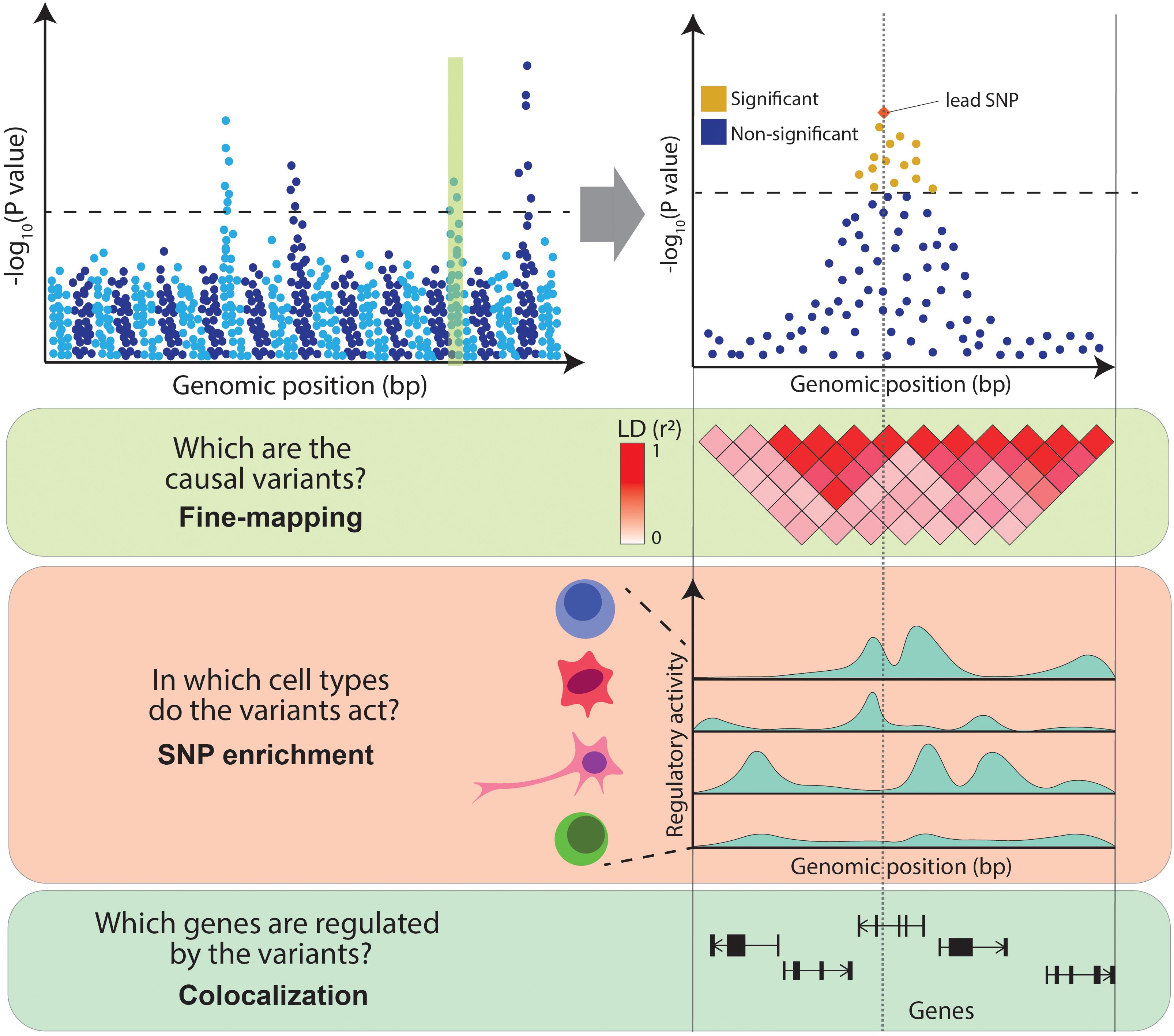
More recent techniques in gene mapping include the so-called genome wide association studies (GWAS) that can identify genes in more structured populations such as diversity panels and designed populations (e.g., MAGIC) by proper control of structure using relarionship matrices and principal components methodologies. Latest methodologies bring the benefits of classical composite interval mapping into the GWAS framework. Bioflow currently offers the classical Q+K model popularized by Kang et al. (2008, 2010). In addition to quantitative genetics methodologies, many bioinformatic-based methodologies have been developed to compare genomes across different species and do gene annotation. These second type of methodologies are not within the scope of Bioflow.

References:

Kang et al. 2008. Efficient control of population structure in model organism association mapping. Genetics 178:1709-1723.

Kang et al. 2010. Variance component model to account for sample structure in genome-wide association studies. Nat. Genet. 42:348-354.

Image taken from https://en.wikipedia.org/wiki/Genome-wide_association_study

Genome wide association

Data Status (wait to be displayed):

Load example

Details

The Genome-Wide Association Studies (GWAS) is a popular model that have helped efforts to dissect causal biological mechanisms underlying various agronomically important traits. The way the options are used is the following:

Traits to analyze.- Traits to be analyzed (from STA and MTA modules).

Markers to analyze.- Markers to be analyzed (from filtered markers).

Environments to analyze.- Differents environments to be considered (across for MTA).

Additional settings.-

Model to use.- Whether rrBLUP or gBLUP should be considered.

Print logs.- Whether the logs of the run should be printed in the screen or not.

References

Kinghorn, B. (1999). 19. Mate Selection for the tactical implementation of breeding programs. Proceedings of the Advancement of Animal Breeding and Genetics, 13, 130-133.

https://alphagenes.roslin.ed.ac.uk/wp/wp-content/uploads/2019/05/01_OptimalContributionSelection.pdf?x44213

Woolliams, J. A., Berg, P., Dagnachew, B. S., & Meuwissen, T. H. E. (2015). Genetic contributions and their optimization. Journal of Animal Breeding and Genetics, 132(2), 89-99.

Cano-Gamez, E., & Trynka, G. (2020). From GWAS to function: using functional genomics to identify the mechanisms underlying complex diseases. Frontiers in genetics, 11, 424.

Software used

R Core Team (2024). R: A language and environment for statistical computing. R Foundation for Statistical Computing, Vienna, Austria. URL https://www.R-project.org/.

Boer M, van Rossum B (2022). _LMMsolver: Linear Mixed Model Solver_. R package version 1.0.4.9000.

Covarrubias-Pazaran G. 2016. Genome assisted prediction of quantitative traits using the R package sommer. PLoS ONE 11(6):1-15.

STA/MTA version(s) to analyze

Marker QA version(s) to use

Environment(s) to use

Visual aid (click on the '+' symbol on the right to open)

The visualizations of the input-data located below will not affect your analysis but may help you pick the right input-parameter values to be specified in the grey boxes above.

Trait(s) to analyze

Visual aid (click on the '+' symbol on the right to open)

The visualizations of the input-data located below will not affect your analysis but may help you pick the right input-parameter values to be specified in the grey boxes above.

Trait to visualize

Environment to visualize

Show Genetic marker information

Analysis Name (optional)

Additional model settings...

Model to use

Threshold for significant marker

Print logs?

Download dashboard

What do we mean by mutation history?

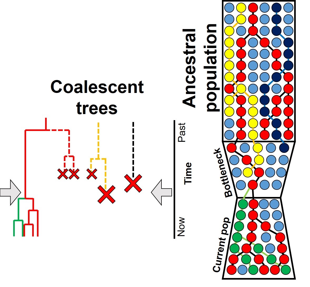
Mutation represents the main source of new variation in DNA-based species in our planet. The accumulation of such mutations tells us about the evolutionary history of species of interest. Many parameters can be of interest for biologists, such as the mutation rate which represents the rate of evolution of species. Other methods to understand evolution linked to mutations are the so-called colascent, which allows to simulate back in the time the evolutionary history.

Currently, Bioflow scope to study mutation is limited to metrics such as mutation rate and hopefully in the future we can add sophisticated methods such as the coalescent.

References:

Wakeley, J. H. (2009). Coalescent theory: an introduction.

Image taken from https://en.wikipedia.org/wiki/Multispecies_coalescent_process

Module under construction.

What do we mean by gene-flow and drift history?

If approached from the evolutionary perspective, the gene flow and drift lead to the formation of new groups that can can result in the development of new species. Is of special interest for evolutionary geneticists to understand the development of these clusters. Some of these methods are normally referred as population-structure based methods. These methods use genotypic or phenotypic information from a set of individuals to understand their level of differentiation and predict future consequences and exploit other charactersitics such as heterosis.

References:

Cavalli-Sforza, L. L. (1966). Population structure and human evolution. Proceedings of the Royal Society of London. Series B. Biological Sciences, 164(995), 362-379.

Image taken from https://en.wikipedia.org/wiki/Population_structure_%28genetics%29

Population structure

Data Status (wait to be displayed):

Details

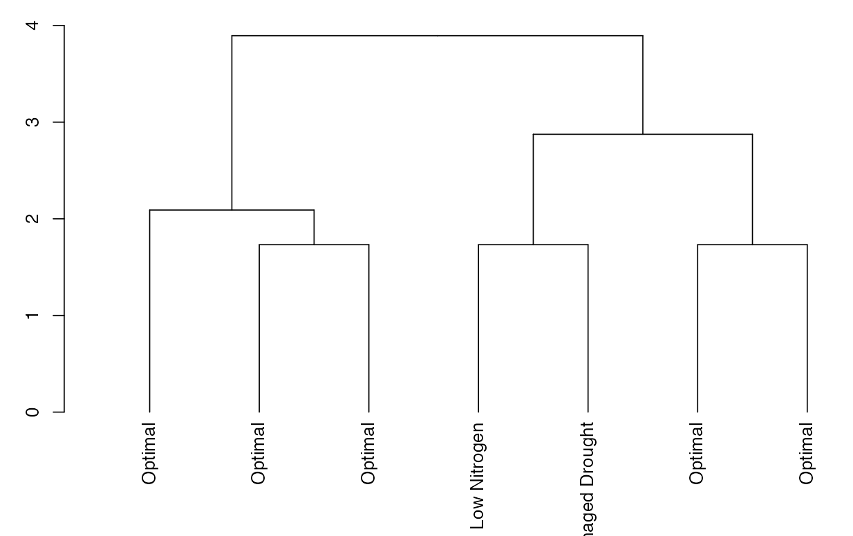
calculate heterozygosity,diversity among and within groups, shannon index, number of effective allele, percent of polymorphic loci, Rogers distance, Nei distance, cluster analysis and multidimensional scaling 2D plot and 3D plot; you can included external groups for colored the dendogram or MDS plots

Add external group.- When you have passport information, you can include this information like a groups. You must load a *.csv file, this should contain in the first column the same names of designation, in the next column the passport information.

Remove monomorphic markers.- When we conform groups by cluster analysis or by external file, this new groups will be contain monomorphics markers, so you can decide if delete or not from the analysis.

No. Clusters.- For the cluster analysis, you must write the number of groups that you need to divide the population.

Genetic distance to be calculate.- You can decide wich genetic distance will be calculate

References

de Vicente, M.C., Lopez, C. y Fulton, T. (eds.). 2004. Analisis de la Diversidad Genetica Utilizando Datos de Marcadores Moleculares: Modulo de Aprendizaje. Instituto Internacional de Recursos Fitogeneticos (IPGRI), Roma, Italia.

QA-geno stamp to apply (optional)

Visual aid (click on the '+' symbol on the right to open)

The visualizations of the input-data located below will not affect your analysis but may help you pick the right input-parameters to be specified in the grey boxes above.

Add external information for groups in csv format (optional)

Browse...

Load example

Remove monomorphic markers from groups (optional)

No. Clusters (default)

Genetic distance to be calculate

Rogers

Nei

Analysis Name (optional)

Download dashboard

By Genotypes

By Markers

Heatmap Distance Matrix

Scale color

Statiscs of diversity

Dendogram

Size cluster line

Size labels

Spaces

Position legend

Type

Choose a color

Factors and Groups

2D-Plot

X Variable

Y Variable

Choose a color

Plot Title

Title Color

Title Size

Axes color

Axes Label Size

Plot Background color

Points size

AMOVA

Module under construction.

Module under construction.

Module under construction.

Marker-Assisted Hybridity Verification Module

Data Status (wait to be displayed):

Load example dataset

Details

The availability of genetic markers allow a more accurate quality assurance of crosses of different kind (e.g., F1, BCn). This module allows to use the genetic data to perform this QA/QC:

Markers to be used.- selection of genetic markers to be used for the verification process.

Columns to define the expected genotypes.- columns that define the expected genotype.

Ploidy.- number of chromosome copies. This value is important to compute some of the paramters. Default is 2 or diploid.

References

Tukey, J. W. (1977). Exploratory Data Analysis. Section 2C.

Velleman, P. F. and Hoaglin, D. C. (1981). Applications, Basics and Computing of Exploratory Data Analysis. Duxbury Press.

QA-geno stamp(s) to apply

Visual aid (click on the '+' symbol on the right to open)

The visualizations of the input-data located below will not affect your analysis but may help you pick the right input-parameters to be specified in the grey boxes above.

Marker(s) to use

Select all markers?

Visual aid (click on the '+' symbol on the right to open)

The visualizations of the input-data located below will not affect your analysis but may help you pick the right input-parameter values to be specified in the grey boxes above.

Markers to display

Genetic unit(s) to average for expected genotype

Ploidy of the organism

Visual aid (click on the '+' symbol on the right to open)

The visualizations of the input-data located below will not affect your analysis but may help you pick the right input-parameter values to be specified in the grey boxes above.

Analysis Name (optional)

Download dashboard

Progeny

Markers to display

Matrix to plot

Number of genotypes

Number of markers

Dashboards

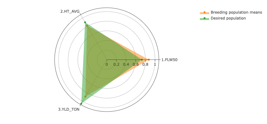
This section has been developed to help the users rebuild their dashboards from previous analysis (e.g., analytical modules), or to combine a set of analysis to create summary dashboards (e.g., ABI dashboards). These graphical representations of the data should allow scientists to understand better their experiments and extract value to help the decision making.

Currently, Bioflow has only two stakeholders that have requested a summary dashboard of breeding pipelines to create show some metrics. If more are needed please contact us.

References:

Image taken from https://stackoverflow.com/tags/plotly/info

Report Reconstruction Module

Data Status (wait to be displayed):

Load example data

Details

This module has the sole purpose of rebuilding the dashboard reports when the user loads an analysis object and doesn't require to re-run an analysis. The idea is that the user only has to specify the analysis type and time stamp and this should suffice. The arguments are used in the following way:

Module report- This argument is used to subset the time stamps to specific type of analyisis. For example, if 'sta' is selected only time stamps associated to sta analysis will be displayed in the next argument. .

Time stamp- This is a dropdown menu that contains the times stamps associated to the analysis type selected.

References

Tukey, J. W. (1977). Exploratory Data Analysis. Section 2C.

Velleman, P. F. and Hoaglin, D. C. (1981). Applications, Basics and Computing of Exploratory Data Analysis. Duxbury Press.

Pick module and timestamp
Build dashboard

Module report

Time stamp

Visual aid (click on the '+' symbol on the right to open)

The visualizations of the input-data located below will not affect your analysis but may help you pick the right input-parameters to be specified in the grey boxes above.

Download dashboard

Accelerated Breeding Dashboard Module

Data Status (wait to be displayed):

Load example data

Details

This module has the sole purpose of building a dashboard report for the Accelerated Breeding Initiative (ABI). The idea is that the user only has to specify the OCS and RGG analysis time stamps requested and a search for all needed metrics by ABI will be executed to build the desired dashboard. The arguments are used in the following way:

Time stamp- This is a dropdown menu that contains the times stamps associated to the analysis type selected.

References

Tukey, J. W. (1977). Exploratory Data Analysis. Section 2C.

Velleman, P. F. and Hoaglin, D. C. (1981). Applications, Basics and Computing of Exploratory Data Analysis. Duxbury Press.

Pick time stamps
Build dashboard

OCS analysis (to trace selection history)

RGG analysis (to link gain)

Visual aid (click on the '+' symbol on the right to open)

The visualizations of the input-data located below will not affect your analysis but may help you pick the right input-parameters to be specified in the grey boxes above.

Dashboard

Download dashboard

On Farm Trial Analysis Module

Data Status (wait to be displayed):

Load example dataset

Details

Given the high yield gap between controlled conditions on experimental stations and farmers’ fields, the best hybrids need to be evaluated under farmers’ conditions, together with appropriate commercial benchmark hybrids and internal checks. The On-Farm Trials (OFT) are implemented in collaboration with partners from national agricultural research systems (NARS), seed companies, and non-governmental organizations (NGOs). The overall goal of the On-Farm Trials is to assess the performance of a set of new varieties, which are selected from a rigorous stage-gate advancement process, under farmers’ conditions to identify promising hybrids that perform well under farmers’ conditions before these are announced to the partners for further uptake. The way the options are used is the following:

Trait(s) to include.- Traits to be included in the dashboard. It only includes analyzed traits from sta.

Year of origin.- The name of the column containing the year when the genotype originated.

Entry type.- The name of the column containing the labels of the genotype category (check, tester, entry, etc.).

iBlock.- The name of the column containing the farm information.

Major Diseases.- The name of the column containing whether a major disease was observed or not.

Type of Disease.- The name of the column containing the type of major disease observed.

Disease Severity.- The name of the column containing the severity of major disease observed.

Environment(s) to include.- Environments to be included in the dashboard. It only includes analyzed environments from sta.

STA version to use

Visual aid (click on the '+' symbol on the right to open)

The visualizations of the input-data located below will not affect your analysis but may help you pick the right input-parameter values to be specified in the grey boxes above.

Network plot of current analyses available.

Past modeling parameters from STA stamp selected.

STA predictions table to be used as input.

Trait(s) to include

Visual aid (click on the '+' symbol on the right to open)

The visualizations of the input-data located below will not affect your analysis but may help you pick the right input-parameter values to be specified in the grey boxes above.

Metrics associated to the STA stamp selected.

Trait to visualize

Parameter to visualize

Dispersal of predictions associated to the STA stamp selected.

Trait to visualize

Group by

Year of origin

Entry type

iBlock

Visual aid (click on the '+' symbol on the right to open)

The visualizations of the input-data located below will not affect your analysis but may help you pick the right input-parameter values to be specified in the grey boxes above.

Preview of Pedigree data associated to the STA stamp selected.

Preview of Phenotype data associated to the STA stamp selected.

With Disease Information?

Visual aid (click on the '+' symbol on the right to open)

The visualizations of the input-data located below will not affect your analysis but may help you pick the right input-parameter values to be specified in the grey boxes above.

Preview of Phenotype data associated to the STA stamp selected.

Environment(s) to include

Visual aid (click on the '+' symbol on the right to open)

The visualizations of the input-data located below will not affect your analysis but may help you pick the right input-parameter values to be specified in the grey boxes above.

Connectivity between environments.

Trait to visualize

Entry type to visualize

Add connectivity labels?

Add axis labels?

Font size

Analysis Name (optional)

Dashboard

Please download the dashboard below:

Download dashboard

Biometrical Genetics Workflow (bioflow)

Version Control Technology

Developing Environment (IDE)

Data Storage Technology

Deployment Technology

Contributors of Analytical Modules

Team Activities

Team Members across Centers

Contact us

Local installation

How to contribute to bioflow?

Frequently asked questions

Why breeding analytics is important for my breeding program?

What is different between bioflow and other platforms?

Data Retrieval and Saving

Config Server

Authentication

Data Source

Tutorial

Options

Dictionary of terms

Preview of uploaded data (click on the '+' symbol on the right to view)

Preview of uploaded data (click on the '+' symbol on the right to view)

Preview of uploaded data (click on the '+' symbol on the right to view)

Tutorial

Options

Notes:

Preview of uploaded data (click on the '+' symbol on the right to view)

Options

Preview of uploaded data (click on the '+' symbol on the right to view)

Preview of uploaded data (click on the '+' symbol on the right to view)

Options

Preview of uploaded data (click on the '+' symbol on the right to view)

Preview of uploaded data (click on the '+' symbol on the right to view)

Options

Tutorial

Tutorial

What do we mean by quality assurance?

Raw Phenotype Outlier Detection Module

Data Status (wait to be displayed):

Details

References

Visual aid (click on the '+' symbol on the right to open)

The visualizations of the input-data located below will not affect your analysis but may help you pick the right input-parameters to be specified in the grey boxes above.

Genetic Markers Curation Module

Data Status (wait to be displayed):

Details

References

Visual aid (click on the '+' symbol on the right to open)

The visualizations of the input-data located below will not affect your analysis but may help you pick the right input-parameter values to be specified in the grey boxes above.

Additional run settings (optional)...

Trait transformations

Trait Transformation Module

Data Status (wait to be displayed):

Details

References

Software used

Traits available

Single Cross Marker Matrix Building Module

Data Status (wait to be displayed):

Details

Example

References

Software used

Visual aid (click on the '+' symbol on the right to open)

The visualizations of the input-data located below will not affect your analysis but may help you pick the right input-parameters to be specified in the grey boxes above.

Visual aid (click on the '+' symbol on the right to open)

The visualizations of the input-data located below will not affect your analysis but may help you pick the right input-parameters to be specified in the grey boxes above.

Visual aid (click on the '+' symbol on the right to open)

The visualizations of the input-data located below will not affect your analysis but may help you pick the right input-parameters to be specified in the grey boxes above.

What do we mean by quality assurance?

Environment-Pheno Filtering Module

Data Status (wait to be displayed):

Details

References

Settings...

Visual aid (click on the '+' symbol on the right to open)

The visualizations of the input-data located below will not affect your analysis but may help you pick the right input-parameter values to be specified in the grey boxes above.

Experimental Design Factor Filtering Module

Data Status (wait to be displayed):

References

Henderson Jr, C. R. (1982). Analysis of covariance in the mixed model: higher-level, nonhomogeneous, and random regressions. Biometrics, 623-640.
Odegard, J., Indahl, U., Stranden, I., & Meuwissen, T. H. (2018). Large-scale genomic prediction using singular value decomposition of the genotype matrix. Genetics Selection Evolution, 50(1), 1-12.